5. Selecting eligible lapse crosscorrelations
There are two parameters that determine a lapse crosscorrelation’s eligibility when it comes to the determination of \(t^{(+,\mathrm{app})}_{i,j,k} + t^{(-,\mathrm{app})}_{i,j,k}\). The first is the SNR of the causal and acausal interferometric surface waves. The second is the distance between lapse crosscorrelation’s two stations.
[1]:
import matplotlib.pyplot as plt
import ocloc
import pandas as pd
[2]:
# We load everything into our main object that will handle all the operations.
cd = ocloc.ClockDrift(station_file='/Users/localadmin/Dropbox/GitHub/ocloc/tutorials/station_info',
                      path2data_dir='/Users/localadmin/Dropbox/GitHub/data',
                      reference_time = '2014-08-21T00:00:00.000000Z',
                      list_of_processing_parameters=[ocloc.ProcessingParameters()])
No correlation file found for station:O26
No correlation file found for station:#STK
5.1 SNR threshold
The quality of the measurements (i.e., the \(t^{(+,\mathrm{app})}_{i,j,k} + t^{(-,\mathrm{app})}_{i,j,k}\)) strongly depends on the signal-to-noise ratio (SNR). If the SNR is too low, the algorithm will struggle to determine the arrival times of the interferometric responses. To see it more clearly let’s plot a crosscorrelation with a low SNR.
[3]:
cd.plot_correlations_of_stationpair("O21", "O08", max_t=60)
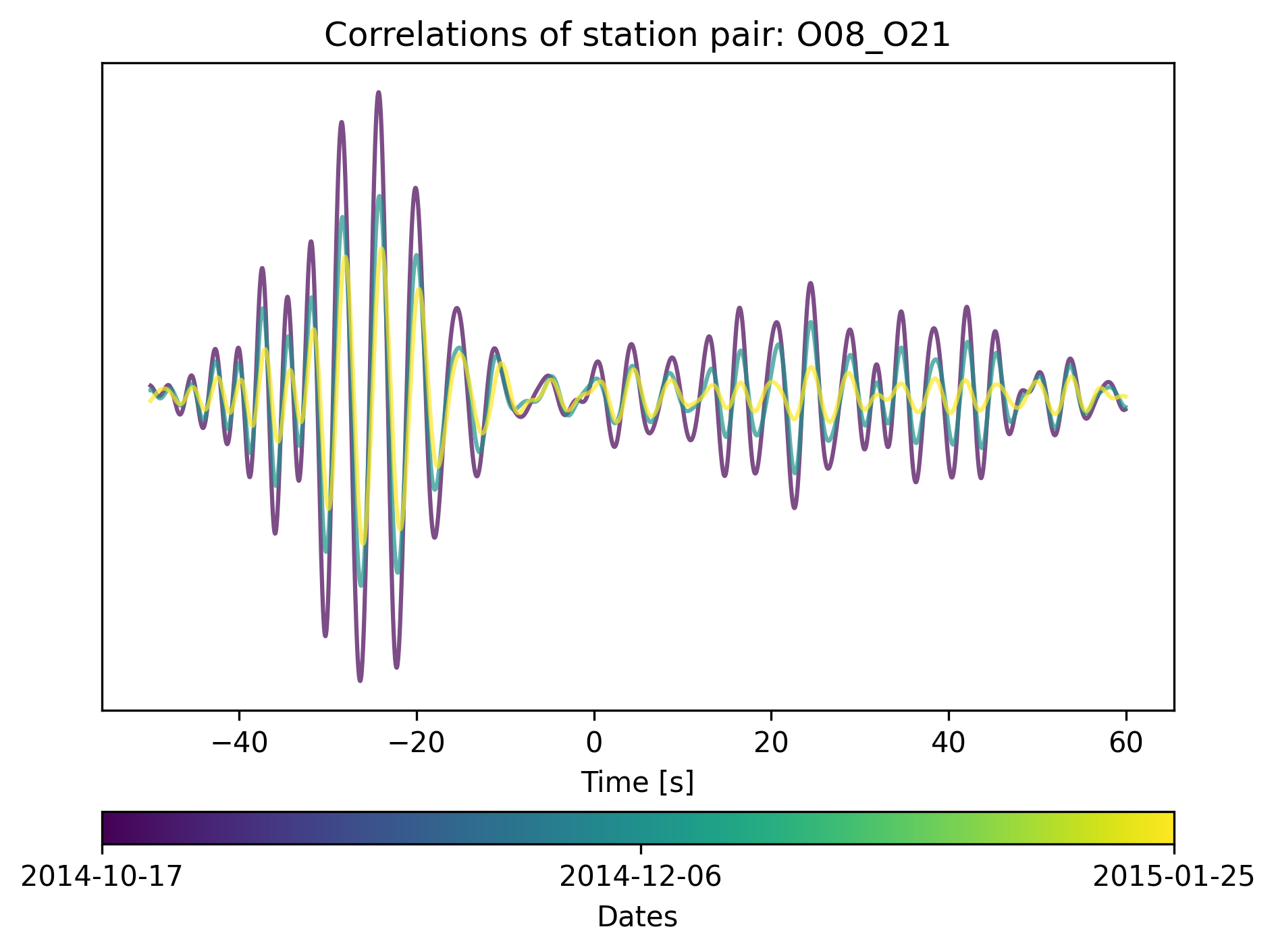
As you can see, the arrival time of the causal wave is not clear. At least for the frequencies we selected. It is important to check these parameters before the inversion.
5.2 Distance threshold
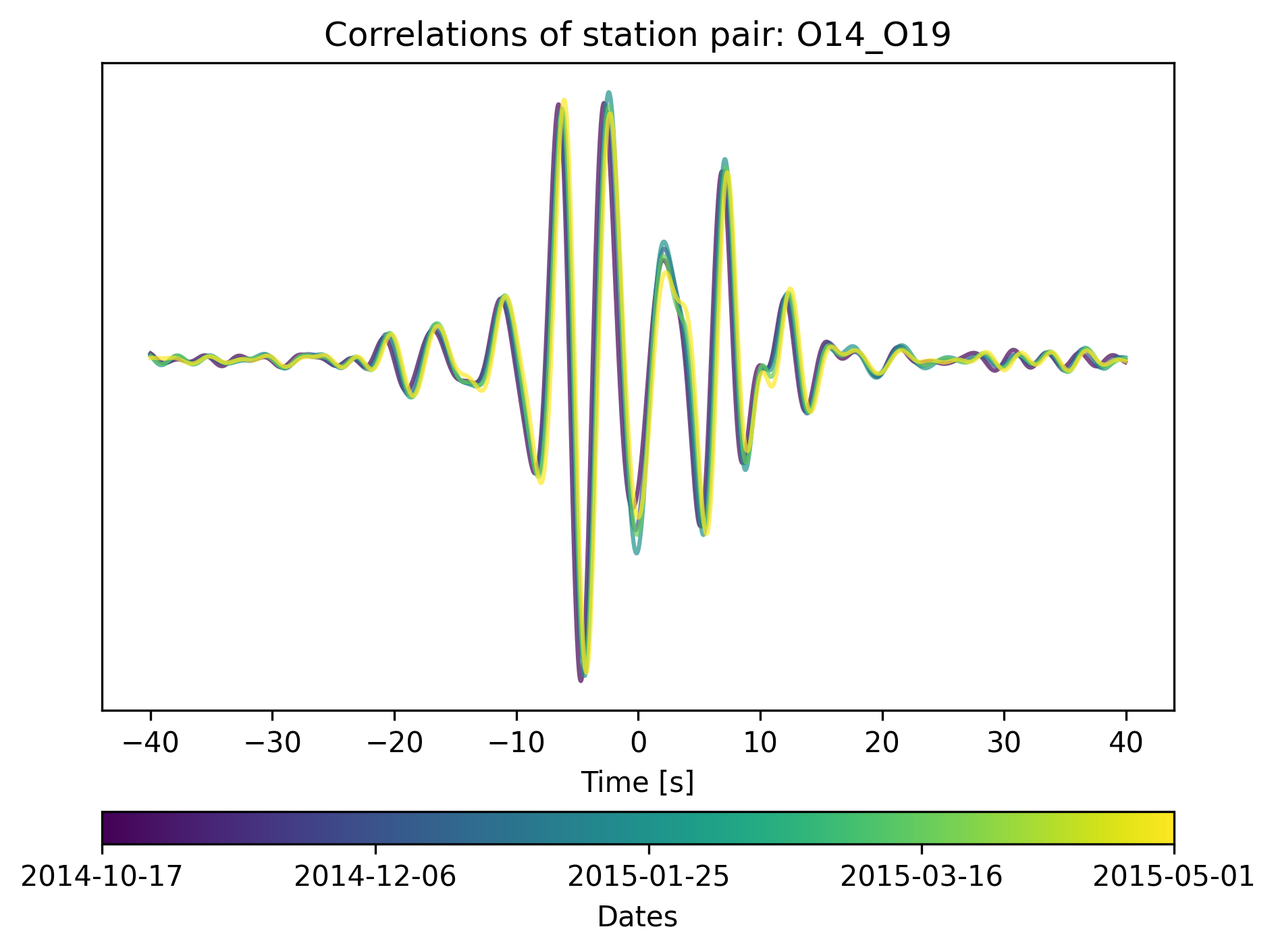
If two stations are too close to each other, the direct surface-wave response at positive time (i.e., the causal arrival) will overlap with the direct surface-wave response at negative time (i.e., the acausal arrival).
[4]:
cd.plot_correlations_of_stationpair("O14", "O19", min_t=-40, max_t=40)
5.3 Removing stations that have crosscorrelations that are not distributed over time.
After calculating the t_app for all crosscorrelations (cd.calculate_tapp_4_allcorrelations()) you can see how well distributed your correlations are over time for a given station. The days_apart argument tells how many days are being grouped together depending on the average time.
For example, let’s assume you have two crosscorrelations where their corresponding average dates are October 5 and October 10. If you set days_apart = 7 the crosscorrelations will be grouped as one correlation period. If you set days_apart = 3, then both will form part of the same group.
[5]:
days_apart = 30
cd.calculate_tapp_4_allcorrelations(days_apart=days_apart)
Calculating the apriori estimates for each stationpair
Calculating the t_app for each stationpair.
You can check the groups of a given station as:
[6]:
station = cd.get_station("O01")
station.no_corr_per_avg_date
[6]:
{'2014-10-17': 27, '2014-12-03': 27, '2015-01-19': 27, '2015-03-16': 26}
[7]:
cd.no_corr_per_avg_date(station=station, days_apart=days_apart, plot=True)
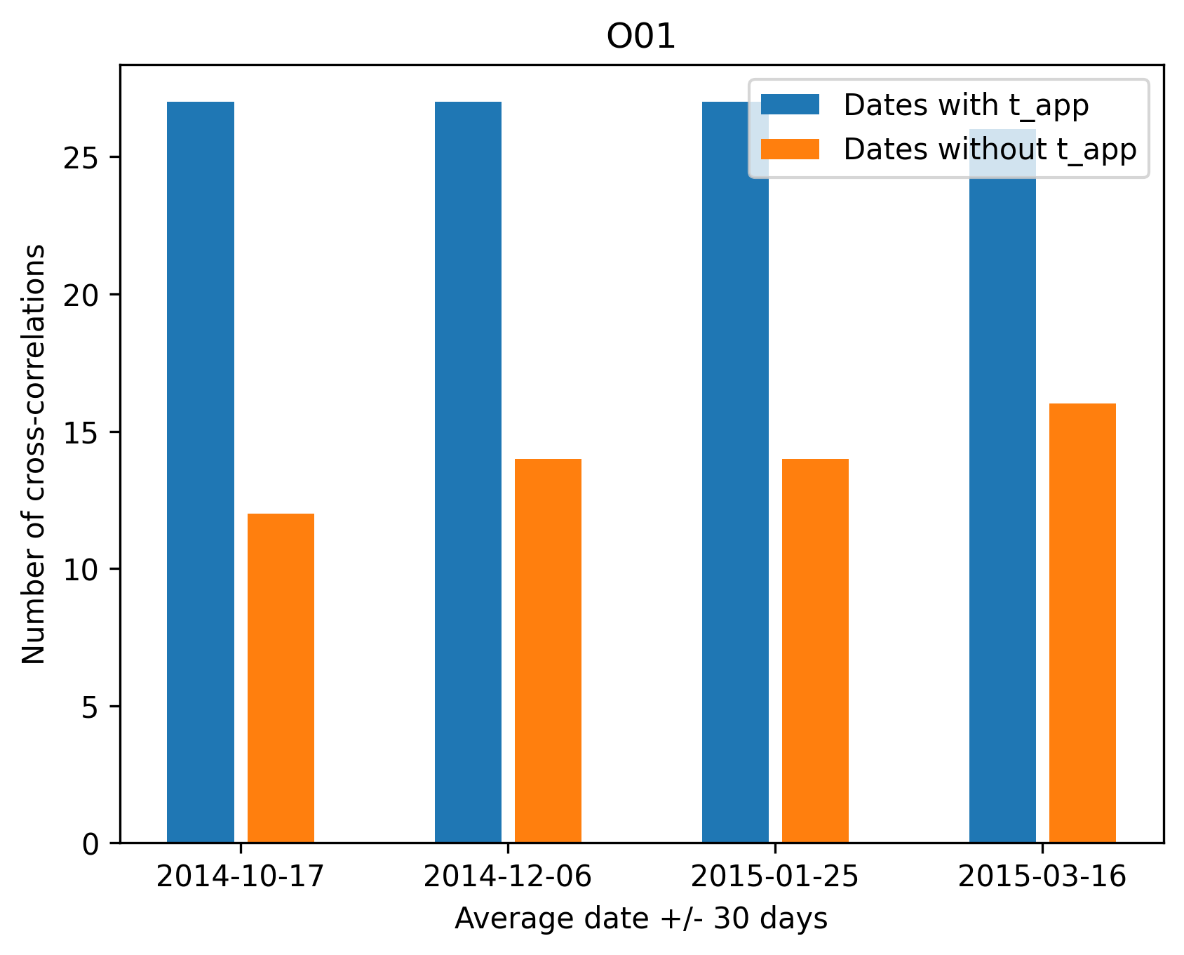
You can also visualize and compare the # of correlations where the program did not find the \(t^{+, app}_{i, j} + t^{-, app}_{i, j}\) as:
It is important to check that we have measures for different time periods because the clock drift depends on the time. Therefore, if we only have points for one single time, then the correction would not be accurate.
For example, let’s take a look at the \(t^{+, app}_{i, j} + t^{-, app}_{i, j}\) of station O01.
[8]:
import seaborn as sns
correlations = cd.get_correlations_of_station("O01")

# Get the average dates and calculate number of dates since reference time.
dates = [(c.average_date-cd.reference_time)/86400 for c in correlations]

# Retrieve the computed $t^{+, app}_{i, j} + t^{-, app}_{i, j}$
t_apps = [abs(c.t_app[-1]) for c in correlations]

# Make it a dataframe and use seaborn for plotting nicely
df = pd.DataFrame(data={'dates': dates, 't_apps': t_apps})
sns.lmplot(x="dates", y="t_apps", data=df);
plt.xlabel("Days since reference time " + str(cd.reference_time)[:10])
plt.show()
/Users/localadmin/Dropbox/GitHub/pip_envs/ocloc_env/lib/python3.8/site-packages/seaborn/axisgrid.py:118: UserWarning: The figure layout has changed to tight
  self._figure.tight_layout(*args, **kwargs)
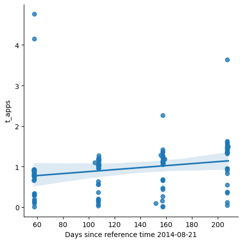
If concentrate all the measurements to the dates between 90 to 120 days after reference_time, then the many lines can be fitted to the data and it yields incorrect results.
Note: The above example includes all the \(t^{+, app}_{i, j} + t^{-, app}_{i, j}\) for one station. Remember that the \(t^{+, app}_{i, j} + t^{-, app}_{i, j}\) is also affected by the time errors of the station with which it is being correlated so a linear regression is not enough to recover the clock errors of a given staiton.
5.4 Removing stations that do not have enough crosscorrelations
Filter stations that don’t have a minimum number of cross-correlations.
Filter stations that have all the crosscorrelations concentrated on a single point in time.
Filter stations that have few connections to toher stations.
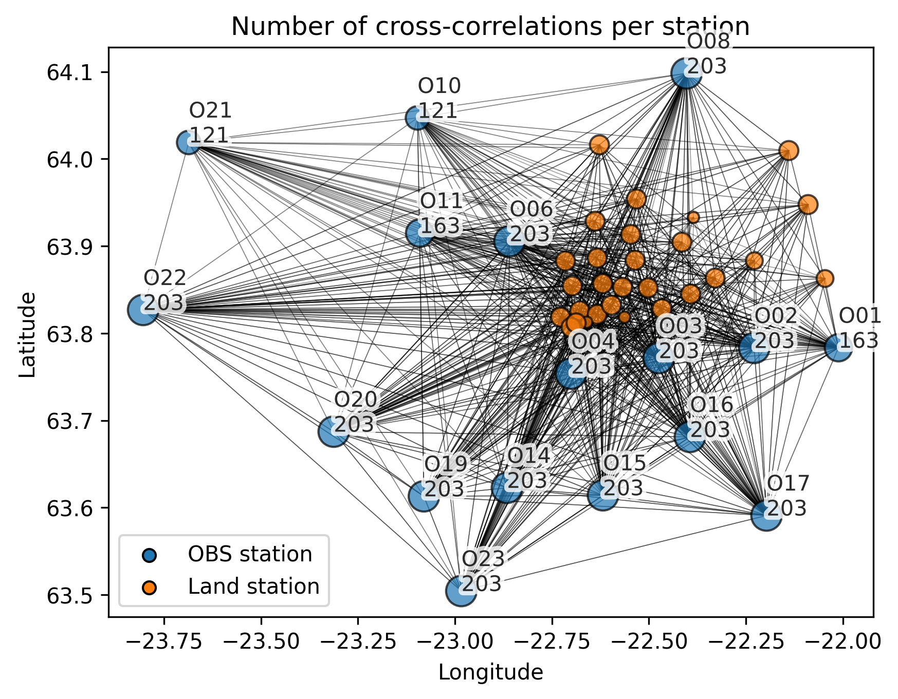
[9]:
cd.plot_inventory_correlations()

[10]:
min_number_of_total_correlations = 2
min_number_correlation_periods = 2
min_number_of_stationconnections = 2

# Number of days can be the oldest average_date - earliest average_date
# divided by 10. The 86400 is to convert from seconds to days.
average_dates = [c.average_date for c in cd.correlations]
days_apart = (max(average_dates) - min(average_dates)) / (5 * 86400)
[11]:
cd.filter_stations(min_number_of_total_correlations,
                   min_number_correlation_periods,
                   min_number_of_stationconnections,
                   days_apart)
[12]:
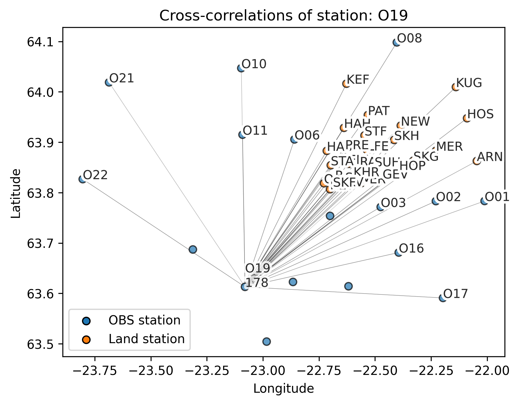
cd.plot_inventory_correlations()
cd.plot_connections_of_station("O19")